PDF

Theranostics 2013; 3(10):802-815. doi:10.7150/thno.5130 This issue Cite

Review

Direct Estimation of Kinetic Parametric Images for Dynamic PET

Guobao Wang, Jinyi Qi

Department of Biomedical Engineering, University of California, Davis, CA 95616.

✉ Corresponding author: qiedu.

Abstract

Dynamic positron emission tomography (PET) can monitor spatiotemporal distribution of radiotracer in vivo. The spatiotemporal information can be used to estimate parametric images of radiotracer kinetics that are of physiological and biochemical interests. Direct estimation of parametric images from raw projection data allows accurate noise modeling and has been shown to offer better image quality than conventional indirect methods, which reconstruct a sequence of PET images first and then perform tracer kinetic modeling pixel-by-pixel. Direct reconstruction of parametric images has gained increasing interests with the advances in computing hardware. Many direct reconstruction algorithms have been developed for different kinetic models. In this paper we review the recent progress in the development of direct reconstruction algorithms for parametric image estimation. Algorithms for linear and nonlinear kinetic models are described and their properties are discussed.

Keywords: Dynamic positron emission tomography, Direct estimation

1 Introduction

1.1 Parametric Imaging with Dynamic PET

Dynamic positron emission tomography (PET) provides the additional temporal information of tracer kinetics compared to static PET. It has been shown that tracer kinetics can be useful in tumor diagnosis such as differentiation between malignant and benign lesions [1, 2], and in therapy monitoring where the kinetic values from dynamic PET can be more predictive for assessment of response than the standard uptake value at a single time point [3, 4].

There are basically two approaches for deriving tracer kinetics from dynamic PET data: region-of-interest (ROI) kinetic modeling and parametric imaging [5-7]. The ROI based approach fits a kinetic model to the average time activity curve (TAC) of a selected ROI, so it is easy to implement and has low computation cost. In contrast, parametric imaging estimates kinetic parameters for every pixel and provides the spatial distribution of kinetic parameters. It is thus more suitable to study heterogeneous tracer uptake in tissue. Parametric images have been found useful in many biological research and clinical diagnosis [8-10]. However, parametric imaging is more demanding computationally and more sensitive to noise in dynamic PET data than the ROI-based kinetic modeling. Obtaining parametric images of high quality therefore raises new challenges that were not faced by conventional ROI-based methods [11].

1.2 Direct Reconstruction of Parametric Images

The typical procedure of parametric imaging is to reconstruct a sequence of emission images from the measured PET projection data first, and then to fit the TAC at each pixel to a linear or nonlinear kinetic model. To obtain an efficient estimate, the noise distribution of the reconstructed activity images should be modeled in the kinetic analysis. However, exact modeling of the noise distribution in PET images can be difficult because noise is spatially variant and object-dependent. Usually the spatial variation and correlations between pixels are simply ignored in the kinetic fitting step, which can lead to very noisy results.

Direct reconstruction has been developed to reduce noise amplification in parametric imaging. Direct reconstruction methods combine tracer kinetic modeling and emission image reconstruction into a single formula to estimate parametric images directly from the raw projection data [12, 13]. Because PET projection data are well-modeled as independent Poisson random variables, direct reconstruction allows accurate compensation of noise propagation from sinogram measurements to the kinetic fitting process. It has been shown that images reconstructed by direct reconstruction methods have better bias-variance characteristics than those obtained by indirect methods for both linear models [33, 34] and nonlinear kinetic models [25, 29].

One drawback of direct reconstruction of parametric images is that the optimization algorithms are more complex than indirect methods [12, 13], due to the intertwinement of the temporal and spatial correlations. In addition, when compartment models are used, the relationship between the kinetic parameters and PET data also becomes nonlinear. Therefore, the development of efficient optimization algorithms for direct reconstruction is of high significance.

1.3 A Brief History of Direct Reconstruction

The theory of direct reconstruction of parametric images was developed right after the publication of the maximum likelihood (ML) expectation-maximization (EM) algorithm for static PET reconstruction [62]. In 1984, Snyder [14] presented an ML EM algorithm to estimate compartmental parameters from time-of-flight list-mode data. Carson and Lange [15] in 1985 presented an EM algorithm for maximum likelihood reconstruction of kinetic parameters from PET projection data. However, neither of these algorithms was validated using a realistic simulation or real data at the time, possibly due to the limitation of computing hardware.

In 1995, Limber et al [16] combined a least squares reconstruction with the Levenberg-Marquardt (LM) algorithm [17] to estimate the parameters of a single exponential decay model from SPECT projection data. Separable nonlinear least squares were used by Huesman et al [18] in 1998 to estimate kinetic parameters of a one-tissue compartment model from 3D SPECT projection data. To reduce computation cost, several researchers also developed methods for direct estimation of kinetic parameters for ROIs instead of reconstruction of the whole parametric images, e.g. [18-22]. These algorithms are only efficient for a small-scale problem with a limited number of ROIs. When the number of unknown parameters goes beyond a few hundreds, both the LM algorithm used by Limber et al [16] and the separable nonlinear least squares used by Huesman et al [18] become inefficient.

The development of algorithms that are suitable for large-scale direct estimation began to attract more and more attention with the recent advances in computing technology. In 2005, a parametric iterative coordinate descent (PICD) algorithm was proposed by Kamasak et al [25] for penalized likelihood estimation of parametric images of a two-tissue compartment model. To our knowledge, this was the first demonstration of direct parametric reconstruction on a dense set of voxels. Yan et al [30] proposed a new EM algorithm for direct ML reconstruction of kinetic parameters of a one-tissue compartment model. Both Kamasak's PICD and Yan's EM algorithms are specific to their respective compartment models. To simplify practical implementation, Wang and Qi in 2008 proposed generalized optimization transfer algorithms for direct penalized likelihood reconstruction of parametric images that are applicable to a wide variety of kinetic models [28, 29]. The algorithms resemble the empirical iterative implementation of the indirect method that alternates between an image reconstruction update and kinetic fitting step (e.g., [26, 27]), but have the advantage of guaranteed monotonic convergence to the direct estimate. Later Wang and Qi [31, 32] also proposed an EM-based optimization transfer algorithm for direct penalized likelihood reconstruction that has faster convergence rate, especially at situations with low background events (randoms and scatters).

Direct reconstruction of parametric images for linear kinetic models has also been developed due to its computational efficiency. In 1997, Matthews et al [23] used the ML EM algorithm to estimate the parametric images of a set of linear temporal basis functions. Meikle et al [24] in 1998 presented a direct reconstruction for the spectral analysis model using the non-negative least squares method. Mathematically, direct reconstruction of linear parametric images is essentially the same as dynamic image reconstruction with overlapping temporal basis functions, such as B-splines [50]. To avoid pre-defined basis functions, Reader et al also proposed a method to estimate the linear coefficients and temporal basis functions simultaneously [53]. To obtain physiologically relevant kinetic parameters directly, Patlak model has been incorporated into direct reconstruction by defining two temporal basis functions as the blood input function and its integral [23]. In 2007, Wang et al [33] presented a maximum a posteriori (MAP) reconstruction of the Patlak parameters using a preconditioned conjugate gradient (PCG) algorithm. Tsoumpas et al [34] presented an ML EM algorithm for direct Patlak reconstruction. Li and Leahy [35], and Zhu et al [36] developed direct reconstruction of the Patlak parameters from list-mode data. Tang et al [37] used anatomical prior information to improve the Patlak reconstruction. Rahmim et al used the AB-EM algorithm [70] to allow negative values in the direct estimation for a Patlak-like graphical analysis model [71]. It has been observed that the strong correlation between the two temporal basis functions in the Patlak model slows down the convergence speed of the direct reconstruction. A nested EM algorithm was developed by Wang and Qi [38] to improve the convergence rate of direct linear parametric reconstruction.

1.4 Aim of This Paper

In this paper we will provide an overview of the recent progress in the development of direct reconstruction algorithms. We will describe technical details of different algorithms and analyze their properties. Methods for direct reconstruction of linear and nonlinear parametric images as well as for joint estimation of parametric images and input function will be included. We expect the information in this review will provide useful guidance to readers for choosing a proper direct reconstruction method.

2 General Formulation of Direct Reconstruction

2.1 PET Data Model

A dynamic PET scan is often divided into multiple consecutive time frames, with each frame containing coincidence events recorded from the start of the frame till the end of the frame. The image intensity at pixel in time frame m, , is then given by

 (1) 

where and denote the start and end times of frame , respectively, and is the decay constant of the radiotracer. is the tracer concentration in pixel at time and is determined by a linear or nonlinear kinetic model with the parameter vector . is the total number of kinetic parameters for each pixel.

Dynamic PET measurements can be well modeled as a collection of independent Poisson random variables [39-42],

 (2) 

where and are the indices of detector pairs and time frames, respectively, and and are the total numbers of the detector pairs and of the time frames, respectively. The expected projection is related to the dynamic image )}, through an affine transform,

 (3) 

 (4) 

where , the th element of the system matrix , is the probability of detecting an event originated in pixel by detector pair , and is the expectation of scattered and random events at detector pair in the th frame. is the total number of image pixels.

Let and be the projection vectors and the image vector in frame . The forward model for time frame can be rewritten in a matrix-vector product form:

 (5) 

Let us define a matrix of kinetic parameters, 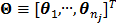, in which each column represents an image of a kinetic parameter. We use to denote its ordered vector. Similarly we also define the following matrices:

and their ordered vectors are denoted by and respectively. Then the expectation of the whole dynamic PET data can be expressed either by

 (6) 

or

 (7) 

where is a identity matrix and denotes the Kronecker product. Equation (6) is the form for practical implementation and equation (7) is more suitable for algorithm analysis.

2.2 Maximum Likelihood Reconstruction

The goal of direct reconstruction is to estimate from dynamic PET measurements. Let denote a set of dynamic PET measurements. and are the matrix and the vector that are formed by in the same fashion as and , respectively. The log Poisson likelihood function of the dynamic PET data is

 (8) 

 (9) 

where a constant term is neglected and is defined by

 (10) 

Maximum likelihood (ML) reconstruction finds the solution by maximizing the log likelihood function,

 (11) 

where denotes the feasible set of the kinetic parameters (e.g. satisfying nonnegativity or box constraints). The resulting images from ML reconstruction at convergence are often very noisy because the tomography problem is ill-conditioned. In practice, the true ML solution is seldom being sought. Rather images are regularized either by early termination before convergence or using a penalty function or image prior to encourage spatial smoothness.

2.3 Penalized Likelihood Reconstruction

Penalized likelihood (PL) reconstruction (or equivalently maximum a posteriori, MAP) regularizes the solution by incorporating a roughness penalty in the objective function to encourage spatially smooth images. PL reconstruction finds the parametric image that maximizes the penalized likelihood function as

 (12) 

where is a smoothness penalty and is the regularization parameter that controls the tradeoff between the resolution and noise. If is too small, the reconstructed image approaches the ML estimate and becomes very noisy; if is too large, the reconstructed image becomes very smooth and useful information can be lost.

The smoothness penalty can be applied either on the kinetic parameters or on the dynamic image , depending on the application. A penalty applied on the dynamic images can be expressed by

 (13) 

where is a smoothness penalty given by

 (14) 

and is the potential function. denotes the neighborhood of pixel ; is the weighting factor equal to the inverse distance between pixels and . A typical neighborhood includes the eight nearest pixels in 2D and 26 nearest voxels in 3D.

The basic requirement of is that it is even and non-decreasing of . A common choice in PET image reconstruction is the quadratic function [42]. The disadvantage of the quadratic regularization is that it can over-smooth edges and small objects when a large is used. To preserve edges, non-quadratic penalty functions can be used. Examples includes the absolute value function , the Lange function 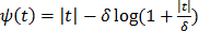[47], and other variations [45, 46]. Nonconvex penalty functions can also be used to even enhance edges, but they are much less popular because the resulting objective function may have multiple local optima.

3 Reconstruction of Parametric Images for Linear Kinetic Models

3.1 Linear Kinetic Models

One way to represent time activity curves is to use a set of linear temporal basis functions. The tracer concentration at time t can be described by,

 (15) 

where is the total number of basis functions, is the th temporal basis function and is the coefficient to be estimated.

The temporal basis functions can be divided into two categories. The first category primarily focuses on efficient representation of time activity curves. Examples include B-splines [48-50] and wavelets [51], as well as those obtained from principal component analysis [52] or adaptively estimated from PET data [53]. One advantage of these basis functions is that they can represent a wide variety of time activity curves. A disadvantage is that the associated coefficients are not directly related to the kinetic parameters of physiological interest. Kinetic modeling is often required to estimate kinetic parameters from the TACs after reconstruction. In comparison, the second category to be described below provides linear coefficients that are directly related to the kinetic parameters of interest.

3.1.1 Spectral Analysis

In spectral analysis the basis functions are a set of pre-determined exponential functions convolved with the blood input function [54, 55],

 (16) 

where denotes the rate constant of the th spectrum and '' represents the convolution operator. The exponential spectral bases are consistent with the compartmental models and the distribution volume (DV) of a reversible tracer can be directly computed from the spectral coefficients by

 (17) 

If the blood input function in (16) is replaced by a reference region TAC , the calculated quantity from the spectral coefficients then becomes the distribution volume ratio (DVR), which is related to binding potential (BP), a major parameter of interest in neuroreceptor studies, by

 (18) 

3.1.2 Patlak Model

The Patlak graphical method [56] is a linear technique which has been widely used in dynamic PET data analysis. For a tracer with an irreversible compartment, the time activity curve satisfies the following linear relationship at the steady state:

 (19) 

where is the time for the tracer to reach steady state. The Patlak slope represents the overall influx rate of the tracer into the irreversible compartment and has found applications in many disease studies. For example, is proportional to the glucose metabolic rate in FDG scans. In some applications, the plasma input function can also be replaced by a reference region input function .

Equation (19) can be rewritten into the following linear model:

 (20) 

where and the two basis functions are

 (21) 

 (22) 

3.1.3 Logan Plot and Relative Equilibrium Plot

For reversible tracers, the Logan plot can be used to estimate distribution volume or binding potential [72]. The standard Logan plot equation is

 (23) 

However, the tissue activity curve is involved nonlinearly in the Logan plot (and also in the multilinear model by Ichise et al [73]), which makes direct reconstruction more difficult. Considering the fact that the ratio between the tissue time activity and plasma concentration remains constant at relative equilibrium, Zhou et al [74] proposed replacing in the denominators by . The model is referred to as the relative equilibrium (RE) model. After a slight rearrangement, we can write the RE model in the following form:

 (24) 

where the cumulative time activity is expressed as a linear combination of the same two basis functions as those in the Patlak plot.

To use the RE model, all the time frames should start from so that the reconstructed dynamic images represent the cumulative time activity . One consequence is that the projection data in different frames are no longer independent, so the likelihood function in (9) needs some modification to obtain a true ML estimate. In addition, the intercept in Eq. (24) is usually negative, which makes the classic EM algorithm not applicable to the resulting direct reconstruction.

Taking the derivative on both sides of (24), Zhou et al [75] presented an alternative form of the RE model,

 (25) 

where is the first-order derivative of . One advantage of the modified RE model in (25) is that it does not involve the cumulative time activity. In addition, since both and are negative, we can rewrite (25) in positive terms

 (26) 

with 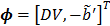and the two basis functions

 (27) 

 (28) 

The model equation (26) is now suitable for direct reconstruction using the classic EM algorithm because the coefficient and the basis function are both nonnegative when . Note that can also be replaced by a reference region TAC to calculate DVR.

3.2 Forward Projection

With a linear kinetic model in (15), the dynamic PET images can be expressed in a matrix-vector product

 (29) 

or equivalently,

 (30) 

where the th element of the temporal basis matrix is given by

 (31) 

Substituting the above equations into Eq. (6), we get the following forward model for the linear kinetic model:

 (32) 

or equivalently,

 (33) 

3.3 Direct Reconstruction Using a Single System Matrix

By treating as a single system matrix , any existing algorithms for static PET reconstruction can be used for the direct estimation of nonnegative linear parametric images. For example, applying the ML EM algorithm [61-63], we get the following update equation for direct linear parametric image reconstruction [23]:

 (34) 

where the superscript denotes the th iteration and

 (35) 

 (36) 

Similar to static PET reconstruction, the convergence of the parametric EM algorithm can be very slow. Preconditioned conjugate gradient (PCG) algorithm and other accelerated algorithms [57, 58] can be used to achieve a faster convergence. One example of direct application of PCG to Patlak reconstruction can be found in [33]. When negative values are present in the parametric images, such as those in the original relative equilibrium model (24), the AB-EM algorithm can be used [71].

One disadvantage of direct reconstruction using a single system matrix is that the convergence can be extremely slow when the temporal basis functions are highly correlated as in the spectral analysis and Patlak model [12]. This is because the combination of the temporal correlation and high spatial dimension results in an ill-posed problem that is much worse than the static PET reconstruction. One way to solve this problem is to decouple the spatial image update and temporal parameter estimation at each iteration using the nested EM algorithm described below.

3.4 Nested EM Algorithm

The nested EM algorithm [38] at iteration first calculates an intermediate dynamic image by

 (37) 

and then updates the kinetic parameter estimate by another EM-like equation

,  (38) 

where , , and is the sub-iteration number in iteration . Each full iteration of the nested EM algorithm consists of one iteration of EM-like emission image update (37) and multiple iterations of kinetic parameter estimation (38).

The nested EM algorithm was derived by using the optimization transfer principle [60]. A surrogate function is constructed at each iteration,

 (39) 

 (40) 

where is given by (37). This surrogate function satisfies

 (41) 

Then the maximization of the original likelihood function is transferred into the maximization of the surrogate function that can be solved pixel-by-pixel,

 (42) 

Applying the EM algorithm to (42) results in the update equation in (38). The property of the surrogate function guarantees

 (43) 

and converges to the global solution.

It is easy to verify that the traditional EM algorithm in (34) is a special case of the nested EM algorithm with [38]. By running multiple iterations of (38) with , the nested EM algorithm can substantially accelerate the convergence rate of the direct reconstruction of linear parametric images without affecting the overall computational time as the size of matrix is much smaller than that of the system matrix . 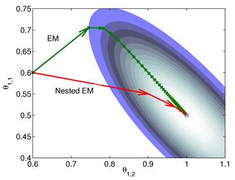This is clearly demonstrated by a toy example shown in Fig. 1 [38]. Starting from the same initial image, the nested EM takes 6 iterations to converge to the true solution, while the traditional EM requires more than 60 iterations. The nested EM algorithm can be further accelerated by considering the nested EM algorithm as an implicit preconditioner and using conjugate directions [38].

 Figure 1 

Isocontours of the likelihood function of a toy problem and the trajectories of the iterates of the traditional EM and the nested EM . The nested EM takes 6 iterations to converge to the final solution, while the traditional EM requires more than 60 iterations. Reprinted from [38] with permission.

4 Reconstruction of Parametric Images for Compartment Models

4.1 Compartment Modeling

While linear models are advantageous for computational efficiency, nonlinear kinetic models based on compartment modeling are more related to the well-developed biochemical kinetics [5]. Under a compartment model, the total tracer concentration in tissue is

 (44) 

where is the fractional volume of blood, is the whole blood concentration, and represents the concentration of the th tissue compartment. The compartment concentrations are related with each other by a set of ordinary differential equations [5, 7],

 (45) 

where , and are the kinetic parameter matrices that are formed by the rate constants in , and denotes the system input.

Taking the Laplace transform of (45), we get

 (46) 

where and denote the Laplace transforms of and , respectively. Then solution of the differential equation (45) can be obtained by

 (47) 

where denotes the inverse Laplace transform.

For the commonly used two-tissue compartment model, we have

 (48) 

and

,  (49) 

with , where are the tracer rate constants, and are the concentrations in the free and bound compartments, and is the tracer concentration in plasma. The analytical solution of is given by

 (50) 

where with , and “*” denotes the convolution operator.

4.2 Model-dependent Algorithms

4.2.1 PICD Algorithm

The parametric iterative coordinate descent (PICD) algorithm [25] was the first direct reconstruction algorithm implemented for a large-scale parametric reconstruction with a compartment model. It first transforms the rate constants in the compartment model into a set of auxiliary parameters and then estimates the auxiliary parameters directly from the sinogram data. For example, the TAC in a two-tissue-compartment model is rewritten as

 (51) 

where the auxiliary parameters are . Once the auxiliary parameters are estimated, the kinetic rate constants can be calculated by

 (52) 

 (53) 

 (54) 

 (55) 

To estimate the auxiliary parameters, a coordinate descent (CD) algorithm is used. The original log-likelihood function is approximated by its second-order Taylor expansion. At each iteration, the auxiliary parameters are updated by

 (56) 

where 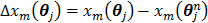, and denote the gradient and Hessian of the negative log-likelihood function with respect to at 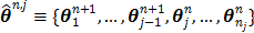and are given by

 (57) 

 (58) 

The first-order derivative and second-order derivative are respectively given by

 (59) 

 (60) 

The regularization term equals to with fixed at for all pixels other than pixel .

The PICD algorithm uses an iterative gradient descent algorithm to update the linear parameters in and an iterative golden section search to estimate the nonlinear components. To accelerate the convergence rate and reduce computational cost, the PICD algorithm updates the linear parameters more frequently than the nonlinear parameters.

The PICD algorithm is well suited for one- and two-tissue-compartment models. For kinetic models with more than two tissue compartments, however, the parameter transformation becomes too complicated.

4.2.2 PMOLAR-1T Algorithm

The PMOLAR-1T algorithm [30] is an EM algorithm for direct reconstruction of parametric images for the one-tissue compartment model. It is derived by introducing a new set of complete data that simultaneously decouples the pixel correlation as well as the temporal convolution. Here we introduce it using the optimization transfer framework.

First we note that the surrogate function in (40) is applicable to any kinetic models. For the one-tissue-compartment model, the tissue time activity curve can be described by

 (61) 

and we have

 (62) 

where . Here we approximate the convolution integral using the summation over uniformly sampled time points with being the time interval.

Applying the EM surrogate function to (40) one more time to decouple the temporal correlation, we can find the maximum of (40) iteratively by

 (63) 

where and is given by

 (64) 

For the one-tissue compartment model with , the optimization in (63) has the following analytical solution:

 (65) 

 (66) 

where is the inverse function of the function [30]

 (67) 

and can be calculated by a look-up table.

The original PMOLAR-1T algorithm [30] only uses one subiteration with . Based on our experience with the nest EM algorithm for linear models, we expect that the convergence rate of the PMOLAR-1T algorithm can be accelerated by using more than one subiterations .

4.3 Model-independent Algorithms

4.3.1 Iterative NLS Algorithms

Reader et al [26] proposed an iterative nonlinear least squares (NLS) algorithm for direct parametric image reconstruction. It iteratively applies the NLS kinetic fitting following an EM image update:

 (68) 

where is the dynamic image given in (37). The weighting factor has to be chosen empirically. In [26] a uniform weight was used. Based on the fact that (40) resembles a Poisson log-likelihood function, Matthews et al [27] proposed the following nonuniform weighting factor

 (69) 

which substantially improved performance over the uniform weight.

However, neither the uniform nor the nonuniform weights provides any theoretical guarantee of convergence because the quadratic function in (68) is not a proper surrogate function. It has been observed that the uniform weight can result in non-monotonic changes in the likelihood function, although the results with the nonuniform weighting are reasonably good.

4.3.2 OT-SP Algorithm

To obtain a guaranteed convergence while maintaining the simplicity of the iterative NLS algorithm, Wang and Qi [29] proposed a quadratic surrogate function for the penalized likelihood function using optimization transfer (OT). The surrogate function of the log-likelihood is derived based on the fact that the second-order derivative of is a non-decreasing function of and is bounded when . The potential function in (14) also has a bounded, non-increasing second-order derivative of . Omitting the constants that are independent of , the surrogate function of the penalized likelihood is given by

 (70) 

where the optimum curvature is set to [43, 44]

 (71) 

with and is an intermediate dynamic sinogram at iteration ,

 (72) 

The second term in (70) is the surrogate function for the penalty function and is given by

 (73) 

where is the optimum curvature of the penalty function

 (74) 

For example for the quadratic penalty and for the nonquadratic Lange penalty.

With , the surrogate satisfies the following condition:

 (75) 

Hence it minorizes the original objective function .

The optimization of the quadratic surrogate function can be solved pixel-by-pixel in a coordinate descent (CD) fashion[29]. However, the OT-CD algorithm is difficult to parallelize because of the sequential update.

For simultaneous update, Wang and Qi further developed an OT-SP (optimization transfer using separable paraboloids) algorithm [29] that uses separable paraboloids to decouple the correlations between pixels in at each iteration. The overall surrogate function that minorizes the original objective function at iteration n is

 (76) 

where the weighting factor in the separable least squares is

 (77) 

with . The intermediate dynamic image is given by

 (78) 

where is the gradient of with respect to ,

 (79) 

evaluated at .

Because is separable for pixels, maximization of is reduced to a pixel-wise least squares fitting optimization:

 (80) 

which can be solved by any existing nonlinear least squares methods (e.g. the Levenberg-Marquardt algorithm).

In summary, each iteration of the OT-SP algorithm consists of two steps: an image update in (78) and a NLS fitting in (80). It has the simplicity of the iterative NLS algorithm, but guarantees a monotonic convergence with . Compared to the PICD and OT-CD algorithms, the OT-SP algorithm can be easily parallelized. A disadvantage of the OT-SP is that it requires the background to be positive for the quadratic surrogate function to work, so the convergence rate can be slow when the level of background events is low.

4.3.3 OT-EM Algorithm

The OT-EM (optimization transfer using the EM surrogate) was derived for direct reconstruction under low background levels [31, 32]. It combines the EM surrogate function in (40) for the log-likelihood function and a separable surrogate function for the penalty function. The overall surrogate function is

 (81) 

The optimization of the penalized likelihood function with respect to is transferred into the maximization of the surrogate function , which can be solved by the following small-scale pixel-wise optimization:

 (82) 

A modified Levenberg-Marquardt algorithm was developed to solve this pixel-wise penalized likelihood fitting in [32].

The OT-EM guarantees a monotonic increase in the penalized likelihood following the optimization transfer properties of . It can be much faster than the OT-SP algorithm when the level of background events (scatters and randoms) is low.

5 Joint Reconstruction of Parametric Images and Input Function

In parametric image reconstruction, the blood input function is required to be known a priori. One standard method of measuring blood input is arterial blood sampling, which is invasive and technically challenging. An alternative to arterial sampling is to derive the input function from a blood region or a reference region in a reconstructed image [65]. When the region used for extraction of the input function is of small size, the image-derived input function (IDIF) can be less accurate due to partial volume and other effects. Joint estimation of the input function and parametric images can potentially improve the accuracy of the IDIF as well as the parametric images by fitting the input function and parametric image to the data simultaneously [64, 65].

5.1 General Formulation

Given a set of kinetic parameters, the time activity curve is a linear function of the input function u(t), which can be either the blood input function or a reference tissue function . Let denote the vector of parameters that defines the input function (e.g. the activity values at a set of time points). Then the joint estimation can be formulated as

 (83) 

where denotes the feasible set of and the penalized likelihood function defined in (12) is rewritten here as an explicit function of .

The maximization in (83) can be solved by an alternating update algorithm (e.g. in [66, 69])

 (84) 

5.2 Joint Estimation without an Input Region

One method for joint estimation without an input region was presented by Reader et al [67]. The algorithm was developed for the linear spectral analysis model. It uses the EM algorithm to find the ML estimation of the input function and the linear coefficients from dynamic projection data. Here we introduce it using the optimization transfer principle and describe how to extend it to nonlinear kinetic models.

We use the EM surrogate function in (40) for the log-likelihood function . Here we rewrite it as an explicit function of the input parameters ,

 (85) 

 (86) 

where is given by (37) and is the same as but as an explicit function of . Since is separable for pixels when v is given, the optimization (84) is transferred to

 (87) 

 (88) 

For a linear kinetic model, both above steps can be solved by the EM algorithm with multiple sub-iterations. When only one sub-iteration is used, it is equivalent to the algorithm in [67].

For compartment models, the optimization in (87) can be solved by the modified Levenberg-Marquardt algorithm given in [32]. The update of in (88) can still be solved by the EM algorithm.

5.3 Joint Estimation with an Input Region

One issue with the joint estimation without an input region is that there is an unknown scaling factor on and the linear coefficients in that cannot be determined. The problem can be solved if there is a region in the image that contains purely the input function. Let denote such a region. Then the image intensity at pixel in time frame is

 (89) 

The joint estimation then estimates the kinetic parameters at pixels outside and the time activity curve inside simultaneously.

Using the same paraboloidal surrogate functions for the OT-SP algorithm, the following algorithm can be obtained [68]:

 (90) 

where and are updated in an alternating fashion. for is updated by the Levenberg-Marquardt algorithm. The estimation of in ( (90) is a linear least squares problem that can be solved easily (e.g. by QR decomposition).

6 Examples

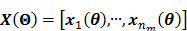
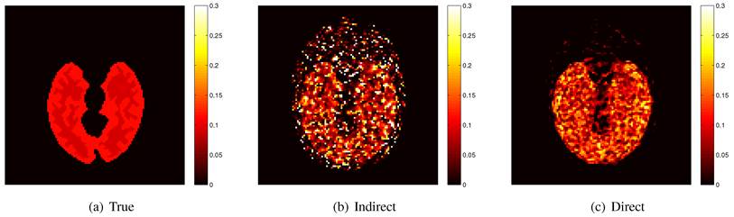
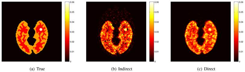
Here we show some simulation results to demonstrate the advantage of direct reconstruction over indirect reconstruction. We simulated a 60-minute F-FDG brain scan using a brain phantom that consisted of gray matter, white matter and a small tumor inside the white matter. The time activity curve of each region was generated using a two-tissue compartment model and an analytical blood input function. Figure 2 shows the images reconstructed by an indirect method and the OT-EM algorithm and Figure 3 shows the corresponding images. Clearly the direct reconstruction results have much less noise than the indirect reconstruction results while maintaining the same spatial resolution. The improvement is similar to those observed in other studies for both linear and compartment models [25, 29, 33].

 Figure 2 

The true and reconstructed images by the indirect and direct algorithms .

 Figure 3 

True and reconstructed images by the indirect and direct algorithms .

7 Conclusion

We have provided an overview of direct estimation algorithms for parametric image reconstruction from dynamic PET data. Because of the combination of tomographic reconstruction and kinetic modeling, direct reconstruction algorithms are more complicated than static image reconstruction. Different algorithms have been developed to balance the tradeoff between simplicity in implementation and fast convergence. We hope that the information in this paper can provide guidance to readers for choosing the proper direct reconstruction algorithm in real applications. In some situations, the choice is clear. For example, the nested EM algorithm should be preferred over the traditional EM algorithm for linear parametric image reconstruction because the former converges much faster while preserving the same simplicity in implementation. In other situations, the choice may be more dependent on the user. We note that as long as the algorithm guarantees global convergence, a simple algorithm can still reach the final solution, albeit with a large number of iterations. We expect that direct parametric image reconstruction will find more and more applications in dynamic PET studies and more novel algorithms will be developed in the future.

Acknowledgements

The authors would like to thank Will Hutchcroft for assistance in typesetting the manuscript.

This work was supported by the National Institute of Biomedical Imaging and Bioengineering under grants R01EB000194 and RC4EB012836 and the Department of Energy under grant DE-SC0002294.

Competing Interests

The authors have declared that no competing interest exists.

References

1. Avril N, Bense S. et al. Breast imaging with fluorine-18-FDG PET: Quantitative image analysis. Journal of Nuclear Medicine. 1997;38(8):1186-1191

2. Dimitrakopoulou-Strauss A, Strauss L.G, Heichel T, Wu H, Burger C, Bernd L, Ewerbeck V. The role of quantitative F-18-FDG PET studies for the differentiation of malignant and benign bone lesions. Journal of Nuclear Medicine. 2002;43(4):510-518

3. Dimitrakopoulou-Strauss A, Strauss L.G, Rudi J. PET-FDG as predictor of therapy response in patients with colorectal carcinoma. Quarterly Journal of Nuclear Medicine. 2003;47(1):8-13

4. Nishiyama Y, Yamamoto Y, Monden T, Sasakawa Y, Kawai N, Satoh K, Ohkawa M. Diagnostic value of kinetic analysis using dynamic FDG PET in immunocompetent patients with primary CNS lymphoma. European Journal of Nuclear Medicine and Molecular Imaging. 2007;34(1):78-8

5. Schmidt K.C, Turkheimer F.E. Kinetic modeling in positron emission tomography. Quarterly Journal of Nuclear Medicine. 2002;46(1):70-85

6. Gunn R.N, Lammertsma A.A, Hume S.P, Cunningham V.J. Parametric imaging of ligand-receptor binding in PET using a simplified reference region model. Neuroimage. 1997;6(4):279-287

7. Gunn R.N, Gunn S.R, Cunningham V.J. Positron emission tomography compartmental models. Journal of Cerebral Blood Flow and Metabolism. 2001;21(6):635-652

8. Kordower J.H, Emborg M.E, Bloch J, Ma S.Y, Chu Y.P, Leventhal L, McBride J, Chen E.Y, Palfi S, Roitberg B.Z, Brown W.D, Holden J.E, Pyzalski R, Taylor M.D, Carvey P, Ling Z.D, Trono D, Hantraye P, Deglon N, Aebischer P. Neurodegeneration prevented by lentiviral vector delivery of GDNF in primate models of Parkinson's disease. Science. 2000;290(5492):767-773

9. Gill S.S, Patel N.K. et al. Direct brain infusion of glial cell line-derived neurotrophic factor in Parkinson disease. Nature Medicine. 2003;9(5):589-595

10. Visser E, Philippens M. et al. Comparison of tumor volumes derived from glucose metabolic rate maps and SUV maps in dynamic 18F-FDG PET. Journal of Nuclear Medicine. 2008;49(6):892-898

11. Zhou Y, Huang S.C, Bergsneider M. Linear ridge regression with spatial constraint for generation of parametric images in dynamic positron emission tomography studies. IEEE Transactions on Nuclear Science. 2001;48(1):125-130

12. Tsoumpas C, Turkheimer F.E, Thielemans K. A survey of approaches for direct parametric image reconstruction in emission tomography. Med. Phys. 2008;35(9):3963-3971

13. A Rahmim, J Tang, H Zaidi. Four-dimensional image reconstruction strategies in dynamic PET: Beyond conventional independent frame reconstruction. Med. Phy. 2009;36(8):3654-3670

14. D. L. Snyder. Parameter-Estimation for Dynamic Studies in Emission-Tomography Systems Having List-Mode Data. IEEE Transactions on Nuclear Science. 1984;31(2):925-931

15. Carson R.E, Lange K. The EM parametric image reconstruction algorithm. Journal of America Statistics Association. 1985;80(389):20-22

16. Limber M.A, Limber M.N, Cellar A, Barney J.S, Borwein J.M. Direct reconstruction of functional parameters for dynamic SPECT. IEEE Transactions on Nuclear Science. 1995;42(4):1249-1256

17. D. W. Marquardt. An algorithm for least-squares estimation of nonlinear parameters. Journal of the Society for Industrial and Applied Mathematics. 1963;11(2):431-441

18. Huesman R.H, Reutter B.W. et al. Kinetic parameter estimation from SPECT cone-beam projection measurements. Physics in Medicine and Biology. 1998;43(4):973-982

19. Zeng G.L, Gullberg G.T, Huesman R.H. Using linear time-invariant system theory to estimate kinetic parameters directly from projection measurements. IEEE Transactions on Nuclear Science. 1995;42(6):2339-2346

20. Reutter B.W, Gullberg G.T, Huesman R.H. Kinetic parameter estimation from attenuated SPECT projection measurements. IEEE Transactions on Nuclear Science. 1998;45(6):3007-3013

21. Chiao P.C, Rogers W.L, Clinthorne N.H, Fessler J.A, Hero A.O, Jones T, Price P. Model-Based Estimation For Dynamic Cardiac Studies Using ECT. IEEE Transactions on Medical Imaging. 1994;13(2):217-226

22. Vanzi E, Formiconi A.R, Bindi D, Cava G.L, Pupi A. Kinetic parameter estimation from renal measurements with a three-headed SPECT system: A simulation study. IEEE Transactions on Medical Imaging. 2004;23(3):363-373

23. Matthews J, Bailey D, Price P, Cunningham V. The direct calculation of parametric images from dynamic PET data using maximum-likelihood iterative reconstruction. Physics in Medicine and Biology. 1997;42(6):1155-1173

24. Meikle S.R, Matthews J.C, Cunningham V.J, Bailey D.L, Livieratos L, Jones T, Price P. Parametric image reconstruction using spectral analysis of PET projection data. Physics in Medicine and Biology. 1998;43(3):651-666

25. Kamasak M.E, Bouman C.A, Morris E.D, Sauer K. Direct reconstruction of kinetic parameter images from dynamic PET data. IEEE Transactions on Medical Imaging. 2005;24(5):636-650

26. Reader A, Matthews J, Sureau F. et al. Iterative kinetic parameter estimation within fully 4D PET image reconstruction. IEEE Nucl. Sci. Syp. & Med. Im. Conf, 3): 1752-56. 2006

27. Matthews J.C, Angelis G.I, Kotasidis F.A, Markiewicz P.J, Reader A.J. Direct reconstruction of parametric images using any spatiotemporal 4D image based model and maximum likelihood expectation maximisation. IEEE Nuclear Science Symposium and Medical Imaging Conference. 2010:2435-2441

28. Wang G, Qi J. Iterative nonlinear least squares algorithms for direct reconstruction of parametric images from dynamic PET. IEEE International Symposium on Biomedical Imaging (ISBI' 08). 2008:1031-1034

29. Wang G, Qi J. Generalized algorithms for direct reconstruction of parametric images from dynamic PET. IEEE Transations on Medical Imaging. 2010;28(11):1717-1726

30. Yan J, Wilson B.P, Carson R.E. Direct 4D list mode parametric reconstruction for PET with a novel EM algorithm. Conference Record of IEEE Nuclear Science Symposium and Medical Imaging Conference. 2008

31. Wang G, Qi J. Direct reconstruction of nonlinear parametric images for dynamic PET using nested optimization transfer. IEEE Nuclear Science Symposium and Medical Imaging Conference, Nov. 2010 (abstract only)

32. Wang G, Qi J. An optimization transfer algorithm for nonlinear parametric image reconstruction from dynamic PET data. IEEE Transations on Medical Imaging. 2012;31(10):1977-1988

33. Wang G.B, Fu L, Qi J.Y. Maximum a posteriori reconstruction of the patlak parametric image from sinograms in dynamic PET. Physics in Medicine and Biology. 2008;53(3):593-604

34. Tsoumpas C, Turkheimer F.E, Thielemans K. Study of direct and indirect parametric estimation methods of linear models in dynamic positron emission tomography. Medical Physics. 2008;35(4):1299-1309

35. Li Q, Leahy R.M. Direct estimation of patlak parameters from list mode PET data. IEEE International Symposium on Biomedical Imaging (ISBI' 09). 2009:390-393

36. Zhu W, Li Q, Leahy R.M. Dual-time-point Patlak estimation from list mode PET data. IEEE International Symposium on Biomedical Imaging (ISBI' 09). 2012:486-489

37. Tang J, Kuwabara H, Wong D.F, Rahmim A. Direct 4D reconstruction of parametric images incorporating anato-functional joint entropy. Physics in Medicine and Biology. 2010;55(15):4261-4272

38. Wang G, Qi J. Acceleration of direct reconstruction of linear parametric images using nested algorithms. Phys Med Bio. 2010;55(5):1505-1517

39. Ollinger J.M, Fessler J.A. Positron-emission tomography. IEEE Signal Processing Magazine. 1997;14(1):43-55

40. Leahy R.M, Qi J.Y. Statistical approaches in quantitative positron emission tomography. Statistics and Computing. 2000;10(2):147-165

41. Lewitt R.M, Matej S. Overview of methods for image reconstruction from projections in emission computed tomography. Proceedings of the IEEE. 2003;91(10):1588-1611

42. Qi J, Leahy R.M. Iterative reconstruction techniques in emission computed tomography. Physics in Medicine and Biology. 2006;51(15):R541-578

43. Fessler J.A, Erdogan H. A paraboloidal surrogates algorithm for convergent penalized-likelihood emission image reconstruction. IEEE Nuclear Science Syposium and Medical Imaging Conference. 1998:1132-5

44. Erdogan H, Fessler J.A. Monotonic algorithms for transmission tomography. IEEE Transactions on Medical Imaging. 1999;18(9):801-814

45. Huber P.J. Robust Statistics. New York, NY, USA: John Wiley & Sons. 1981

46. Bouman C, Sauer K. A generalized Gaussian image model for edge-preserving MAP estimation. IEEE Trans Image Proc. 2002;2(3):296-310

47. K. Lange. Convergence of EM image reconstruction algorithms with Gibbs smoothing. IEEE Trans Med Imaging. 1990;9(4):439-446

48. Reutter B.W, Gullberg G.T, Huesman R.H. Direct least-squares estimation of spatiotemporal distributions from dynamic SPECT projections using a spatial segmentation and temporal B-splines. IEEE Transactions on Medical Imaging. 2000;19(5):434-450

49. Reutter B.W, Gullberg G.T, Huesman R.H. Effects of temporal modelling on the statistical uncertainty of spatiotemporal distributions estimated directly from dynamic SPECT projections. Physics in Medicine and Biology. 2002;47(15):2673-2683

50. Nichols T.E, Qi J, Asma E, Leahy R.M. Spatiotemporal reconstruction of list-mode PET data. IEEE Transactions on Medical Imaging. 2002;21(4):396-404

51. Verhaeghe J. et al. Dynamic PET reconstruction using wavelet regularization with adapted basis functions. IEEE Transactions on Medical Imaging. 2008;27(7):943-959

52. Maltz JS. Optimal time-activity basis selection for exponential spectral analysis: application to the solution of large dynamic emission tomographic reconstruction problems. IEEE Transactions on Nuclear Science. 2001;48(4):1452-1464

53. Reader A.J, Sureau F.C, Comtat C, Trebossen R, Buvat I. Joint estimation of dynamic PET images and temporal basis functions using fully 4D ML-EM. Physics in Medicine and Biology. 2006;51(21):5455-5474

54. Cunningham V.J, Jones T. Spectral-analysis of dynamic PET studies. Journal of Cerebral Blood Flow and Metabolism. 1993;13(1):15-23

55. Gunn R.N, Gunn S.R, Turkheimer F.E. et al. Positron emission tomography compartmental models: A basis pursuit strategy for kinetic modeling. Journal of Cerebral Blood Flow and Metabolism. 2002;22(12):1425-1439

56. Patlak C.S, Blasberg R.G. Graphical evaluation of blood-to-brain transfer constants from multiple-time uptake data generalizations. Journal of Cerebral Blood Flow and Metabolism. 1985:584-590

57. Li Q.Z, Asma E, Ahn S, Leahy R.M. A fast fully 4-D incremental gradient reconstruction algorithm for list mode PET data. IEEE Transactions on Medical Imaging. 2007;26(1):58-67

58. Ahn S, Fessler J.A. Globally convergent image reconstruction for emission tomography using relaxed ordered subsets algorithms. IEEE Transactions on Medical Imaging. 2003;22(5):613-626

59. Fessler J.A, Booth S.D. Conjugate-gradient preconditioning methods for shift-variant PET image reconstruction. IEEE Transactions on Image Processing. 1999;8(5):688-699

60. Lange K, Hunter D.R, Yang I. Optimization transfer using surrogate objective functions. Journal of Computational and Graphical Statistics. 2000;9(1):1-20

61. Dempster A.P, Laird N.M, Rubin D.B. Maximum likelihood from incomplete data via the EM algorithm. Journal of the Royal Statistical Society, Series B. 1977;39(1):1-38

62. Shepp L.A, Vardi Y. Maximum likelihood reconstruction for emission tomography. IEEE Transactions on Medical Imaging. 1982;1(2):113-122

63. Lange K, Carson R.E. EM reconstruction algorithms for emission and transmission tomography. Journal of Computer Assisted Tomography. 1984;8(2):306-316

64. Feng D.G, Wong K.P, Wu C.M, Siu W.C. A technique for extracting physiological parameters and the required input function simultaneously from PET image measurements: Theory and simulation study. IEEE Transactions on Information Technology in Biomedicine. 1997;1(4):243-254

65. Zanotti-Fregonara P, Chen K, Liow J.S, Fujita M, Innis R.B. Image-derived input function for brain PET studies: many challenges and few opportunities. Journal of Cerebral Blood Flow and Metabolism. 2011;31(10):1986-98

66. Yetik I.S, Qi J. Direct estimation of kinetic parameters from the sinogram with an unknown blood function. IEEE International Symposium on Biomedical Imaging (ISBI' 06)): 295-298. 2006

67. Reader A.J, Matthews J.C, Sureau F.C, Comtat C, Trebossen R, Buvat I. Fully 4D image reconstruction by estimation of an input function and spectral coefficients. IEEE Nuclear Science Symposium and Medical Imaging Conference. 2007:3260-3267

68. Wang G, Qi J. Direct reconstruction of PET receptor binding parametric images using a simplified reference tissue model. Proceedings of SPIE Medical Imaging Conference. 2009:V1-V8

69. Kamasak M.E, Bouman C.A, Morris E.D, Sauer K.D. Parametric reconstruction of kinetic PET data with plasma function estimation. SPIE Computational Imaging III. 2005:293-794

70. C. Byrne. Iterative algorithms for deblurring and deconvolution with constraints. Inverse Problems. 1998;14(6):14551467

71. Rahmim A, Zhou Y, Tang J, Lu L, Sossi V, Wong D.F. Direct 4D parametric imaging for linearized models of reversibly binding PET tracers using generalized AB-EM reconstruction. Physics in Medicine and Biology. 2012;57(3):733-755

72. Logan J, Fowler J.S, Volkow N.D, Wolf A.P, Dewey S.L, Schlyer D.J, MacGregor R.R, Hitzemann R, Bendriem B, Gatley S.J, Christman D.R. Graphical analysis of reversible radioligand binding from time-activity measurements applied to [N-11C- methyl]-(-)-cocaine PET studies in human subjects. Journal of Cerebral Blood Flow and Metabolism. 1990;10(5):740-747

73. Ichise M, Liow J.S, Lu J.Q, Takano A, Model K, Toyama H, Suhara T, Suzuki K, Innis R.B, Carson R.E. Linearized reference tissue parametric imaging methods: application to [11C]DASB positron emission tomography studies of the serotonin transporter in human brain. Journal of Cerebral Blood Flow and Metabolism. 2003;23(9):1096-112

74. Zhou Y, Ye W, Brasic J.R, Crabb A.H, Hilton J, Wong D.F. A consistent and efficient graphical analysis method to improve the quantification of reversible tracer binding in radioligand receptor dynamic PET studies. Neuroimage. 2009;44(3):661-670

75. Zhou Y, Sojkova J, Resnick S.M, Wong D.F. Relative Equilibrium Plot Improves Graphical Analysis and Allows Bias Correction of Standardized Uptake Value Ratio in Quantitative 11C-PiB PET Studies. Journal of Nuclear Medicine. 2012;53(4):622-628

Author contact

Corresponding author: qiedu.

Received 2013-1-24
Accepted 2013-8-4
Published 2013-11-20

Citation styles

©2024 Ivyspring International Publisher. Terms of use